Acoustic Hologram Optimisation Using Automatic Differentiation in JAX
On December 2020, Tatsuki Fushimi, Kenta Yamamoto & Yoichi Ochiai have submitted a preprint, later accepted by Scientific Reports, on using automatic differentiation for the optimization of acoustic holograms produced by phased arrays.
In the following, we will implement the main algorithm discussed in the paper using jax: this work provides a good case study for demonstrating the use of jax for scientific applications not related to machine learning.
Problem setup
Assume to have a transducer located in \(x_t\), which is transmitting a monochromatic (single frequency) signal with wavenumber
\[k = \frac{2\pi f_0}{c_0},\]where \(f_0\) is the transmit frequency and \(c_0\) is the speed of sound of the homogeneous medium. Then one can use a simplified version of the Rayleigh integral (see [Sapozhnikov et al., 2015] for a more general discussion) to calculate the pressure field at a location \(x_c\)
\[p_{c,t} = \frac{P_{ref}}{\|x_c - x_t\|}D(\theta)e^{j(k\|x_t-x_c\|+ \phi_t)}\]where \(P_{ref}\) is the pressure amplitude at the transducer, \(\phi_t\) is the phase of the transmit wave and
\[D(\theta) = \frac{2J_1(k r \sin(\theta))}{k r \sin(\theta)}\]is the directivity factor which depends on the angle \(\theta\) between the transducer normal and the vector \(x_t-x_c\). Here, the function \(J_1\) is the Bessel function of the first kind of order 1.
Note that the pressure is expressed as a complex number, as it is customary for time harmonic fields, in order to implicitly define the phase relationships between the field at various locations.
The last step is to use the superposition property deriving from the linearity of the wave equation to sum the contribution of \(M\) transducers in the phased array to the field
\[p(x_c) = \sum_{t=1}^{M} p_{c,t}\]Optimization
All is left to use automatic differentiation is to define a loss function. The authors have chosen to optimize the amplitude \(\|p(x_c)\|\) of the field by matching it against some known positive field \(A(x_c)\). Using a squared error distance, this reduces the loss function to
\[\mathcal L(p) = \frac{1}{|\Omega|}\int_\Omega (A(x) - |p(x)|)^2 dx \propto \sum_{x_c \in X} (A(x) - |p(x)|)^2\]for an appropriate dense set of positions \(X\), which we will take as equispaced points (i.e. pixels) to directly compare the field with a digital image.
Implementation
First of all, let’s import the required libraries:
import jax
from jax import numpy as jnp
from matplotlib import pyplot as plt
Afterwards, we define some parameters that we will use throughout the following sections.
# Free parameters
c0 = 346                # Air speed of sound
f0 = 40e3               # Transmit frequency
radius = 0.005          # Radius of the transducer
z_plane = 0.1           # Distance between transducer and target field
k = 2*jnp.pi*f0/c0      # Wavenumber

# Generating transducer positions
x_pos, y_pos = map(
    lambda x: (x-jnp.mean(x)).flatten()*radius, jnp.indices((32,32))
)
z_pos = x_pos*0         # Tranducers on x_y plane, z = 0
positions = jnp.stack([x_pos, y_pos, z_pos],axis=-1)

# Evaluating normals
normals = (positions*0).at[:,2].set(1.) # All normals along the z axis -> (0,0,1)

# Initializing phases to zero
phases = jnp.zeros((positions.shape[0],))

# Sampling positions at the target plane
x_pos, y_pos = map(
    lambda x: (x-jnp.mean(x)).flatten()*radius/8, jnp.indices((256,256))
)
z_pos = x_pos*0 + z_plane  # Plane parallel to the transducers array
plane_positions = jnp.stack([x_pos, y_pos, z_pos],axis=-1)

# Some helper functions
norm = lambda x: jnp.sqrt(jnp.sum(jnp.abs(x)**2))
avg_norm = lambda x: jnp.sqrt(jnp.mean(jnp.abs(x)**2))
dot = lambda x, y: jnp.sum(x*y)
Forward functions
We can start implementing some functions! While doing that, we can focus on a single transducer and a single target point, as we will parallelize (actually, vectorize) everything later on using jax.vmap.
The first function evaluates the angle \(\theta\) between a transducer normal and a target location, simply by using the arc-cosine of their normalized dot product:
def angle_between(x, y):
    return jnp.arccos(dot(x, y)/(norm(x)*norm(y)))
At this point, we hit the first problem: we need the Bessel function of the first kind of order 1 to evaluate the directivity factor, but it looks like JAX doesn’t have it! However, according to Wikipedia it holds the relationship
\[-J_1(x) = \frac{\partial}{\partial x} J_0(x)\]where \(J_0(x)\) is the Bessel function of the first kind of order 0, which is implemented by jax in jax.numpy.i0. So we can implement the Bessel function of the first kind using autodiff with jax.grad (I’m 99% sure this is correct, but I’m not sure):
def J1(x):
    J0 = lambda x: jnp.i0(-1j*x)
    return -jax.grad(J0)(x).real
At this point, we can write the directivity function \(D(\theta)\) as
def directivity_fun(theta):
    x = k*radius*jnp.sin(theta)
    D_with_nans = 2*J1(x)/x
    return jnp.where(jnp.isnan(D_with_nans), 1., D_with_nans)
Having all the main ingredients setup, we can finally write the function that evaluates the beam-pattern of a single transducer (at a single location)
def p_c(x_c, x_t, normal_vec, phase):
    theta = angle_between(x_c, normal_vec)
    D = directivity_fun(theta)
    dist = norm(x_c - x_t)
    output_phase = jnp.exp(1j*(k*dist + phase))
    return D*output_phase/dist
Vectorization
Adding the contribution of all the transducers can be easily done by vectorizing the function above with respect to the input positions, using jax.vmap, and summing them all:
def p_tot(xc, xt, n, phases):
    return jnp.sum(
        jax.vmap(p_c, (None, 0, 0, 0), 0)(xc, xt, n, phases), 0)
Similarly, we can get the field at all the positions by vectorizing the function above with respect to the target location x_c
pc_vect = jax.vmap(p_tot, (0,None,None,None),0)

def get_hologram(x):
    return jnp.reshape(pc_vect(plane_positions, positions,normals,x), (256,256))
Let’s look at the hologram for the initial, flat phase distribution
p = get_hologram(phases)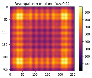
Loss function
Let’s start with a very simple image that we are trying to match
from jax.example_libraries import optimizers
from jax import random

# Constructing reference image
reference_hologram = jnp.zeros((256,256))
reference_hologram = reference_hologram.at[32:64,48:164].set(.5)
reference_hologram = reference_hologram.at[64:200,128:164].set(1.)
reference_hologram = reference_hologram.at[96:128,164:150].set(1.)
reference_hologram = reference_hologram.at[150:210,128:164].set(.3)
reference_hologram = reference_hologram.at[150:190,64:100].set(.7)
reference_hologram = reference_hologram.at[200:230,64:200].set(.2)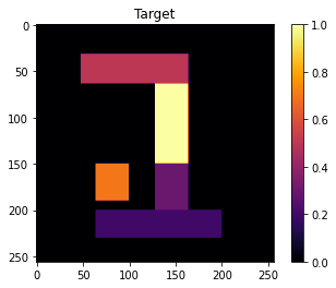
We are going to optimize a slightly different loss function than the Diff-PAT paper, namely the cross correlation, defined as
\[\mathcal L = \sum_i A(x_i) |p(x_i)|\]which is implemented as
def xcorr(a,b):
    return -dot(a,b)/(norm(a)*norm(b))

def lossfun(x):
    return xcorr(jnp.abs(get_hologram(x)), reference_hologram)
Note that the loss function depends on the vector of phases for each transducer. To optimize it, we get the gradient using autodiff
loss_with_grad = jax.value_and_grad(lossfun)Optimization
We are now all setup to optimize the loss function. All we need is an updated function that takes the current vector of phases and updates it using the gradient. We will use the Adam optimizer, as in the Diff-PAT paper.
As it is customary in JAX, we can use the jax.jit to just-in-time compile this function for faster execution.
# Initialize optimizer
init_fun, update_fun, get_params = optimizers.adam(.2)
opt_state = init_fun(phases)

@jax.jit
def update(opt_state, key, iteration):
    params = get_params(opt_state)
    lossval, gradient = loss_with_grad(params)
    return lossval, update_fun(iteration, gradient, opt_state)
All is left to do now is to wrap the update function in a loop that runs for a number of iterations. Note that we explicitly define a random seed for the random number generator, since this aids reproducibility and is anyhow necessary in JAX.
losshistory = []
key = random.PRNGKey(42)

for iteration in range(100):
    _, key = random.split(key)
    lossval, opt_state = update(opt_state, key, iteration)

    # For logging
    losshistory.append(-lossval)
Results
After the optimization is over, which should be relatively fast especially if you are running jax on a GPU, we can visualize the results:
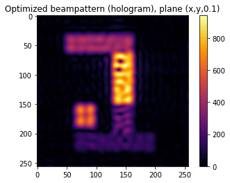
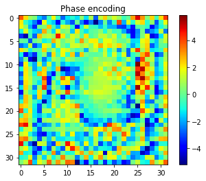
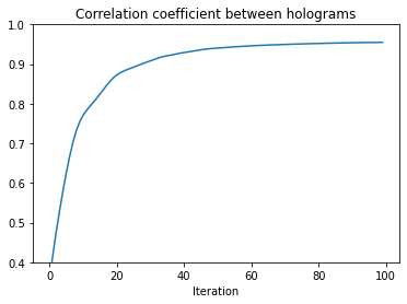
It is fairly close to the target hologram, but not quite. One could experiment with different loss functions, or with different initial phases. Note however that we are currently only controlling the phase of the transducers. If one could also control the amplitude, than the wave propagator is a linear operator of the complex input parameters \(P_{t}e^{j\theta_t}\), making the MSE optimization problem convex and therefore uniquely solvable (up to a global phase shift).
Conclusions
In this tutorial, we have reproduced the Diff-PAT algorithm, and we have shown how JAX can be used to easily and efficiently prototype algorithms that are relevant for numerical physics methods, by exploiting its ability to conveniently transform functions in several ways.
A jupyter notebook implementing this tutorial can be found at the following GitHub repo.
The findings from Fushimi et al. could also be extended in a number of ways. For example, the hologram produced by a planar wavefront could be efficiently propagated in the Fourier domain: this is implemented in the angular_spectrum function of the jwave package.
References
- Fushimi, T., Yamamoto, K. & Ochiai, Y. Acoustic hologram optimisation using automatic differentiation. Sci Rep 11, 12678 (2021). https://doi.org/10.1038/s41598-021-91880-2